When Binomial Distributions Appear Normal

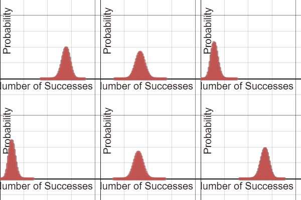
We’re working through binomial and geometric distributions this week in AP Stats, and there are many, many seeds which get planted in this chapter which we hope will yield bumper crops down the road. In particular, normal estimates of a binomial distribution – which later become conditions in hypothesis testing – are valuable to think about now and tuck firmly into our toolkit.  This year, a Desmos exploration provided rich discussion and hopefully helped students make sense of these “rules of thumb”.

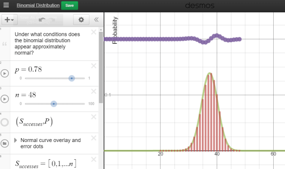
Each group was equipped with a netbook, and some students chose to use their phones. A Desmos binomial distribution explorer I had pre-made was linked on Edmodo. The explorer allows students to set the paremeters of a binomial distribution, n and p, and view the resulting probability distribution. After a few minutes of playing, I asked students what they noticed about these distributions.

A lot of them look normal.

Yup. And now the hook has been cast.  Which of these distributions “appear” normal, and under what conditions?  In their teams, students adjusted the parameters and assessed the normality.  In the expressions, the normal overlay provides a theoretical normal curve, based on the binomial mean and standard deviation, along with error dots. This provides more evidence as students debate normal-looking conditions.

Each group was then asked to summarize their findings:

• Provide 2 settings (n and p) which provide firm normality.
• Provide 2 settings (n and p) which provide a clearly non-normal distribution.
• Optional: provide settings which have you “on the fence”

My student volunteer (I pay in Jolly Ranchers) recorded our “yes, it’s normal!” data, using a second Desmos parameter tracker.  What do we see in these results?

Students quickly agreed that higher sample sizes were more likely to associate with a normal approximation. Now let’s add in some clearly non-normal data dots. After a few dots were contributed, I gave an additional challenge – provide parameters with a larger sample size which seem anti-normal. Hers’s what we saw:

The discussion became quite spirited: we want larger sample sizes, but extreme p’s are problematic – we need to consider sample size and probability of success together!  Yes, we are there!  The rules of thumb for a normal approximation to a binomial had been given in a flipped video lecture given earlier, but now the interplay between sample size and probability of success was clear:

And what happens when we overlay these two inequalities over our observations?

Awesomeness!  And having our high sample sizes clearly outside of the solution region made this all the more effective.

Really looking forward to bringing this graph back when we discuss hypothesis testing for proportions.