Category: Technology

Last spring, the awesome folks at Desmos released a slew of slick (but easy-to-use) statistics features. Here is a brief video I made which walks through a few of the new features. With a new academic year beginning, I’m looking forward to changing some of my classroom moves in AP Stats to leverage the new features and build understanding. Here are 3 moves I’m planning to try this year:

ASSESSING NORMALITY (Here is a previous post on this topic)

Pop quiz! Below you see 6 boxplots. Each boxplot represents a random sample of size 20, each drawn from a large population. Which of the underlying populations have an approximately normal shape? Take a moment to think how you…and your students…might answer…

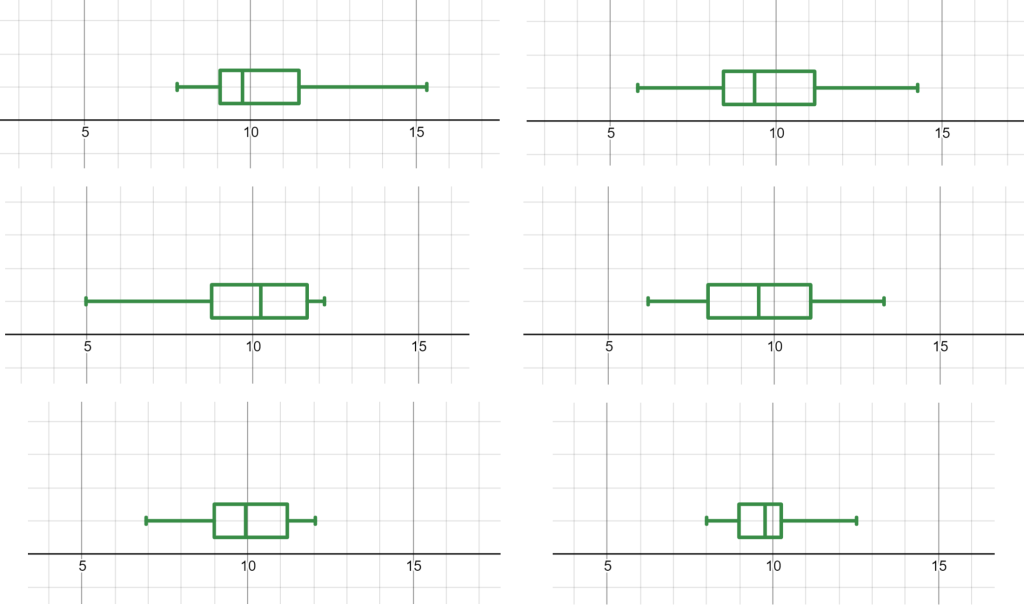
Have your answers ready? Here comes the reveal…..

Not only do each of the samples above come from normal populations, they each come from the same theoretical population! This year in class I plan to walk students through how to build their own random sampler on Desmos, which takes only a few intuitive commands. When the “random” command is used, we now get a re-randomize” button which allows students to cycle through many random samples and assess the shapes. You can toy with my graph here.

Often students look for strict symmetry or place too much stock in different-sized tails. This is a great opportunity to have students explore and understand the variability in sampling. Teach your students to widen their nets when trying to assess normality and remember – our job is usually not to “prove” normality; instead, these samples show that the assumption of population normality is often safe and reasonable, especially with small samples.

LINEAR TRANSFORMATIONS OF DATA

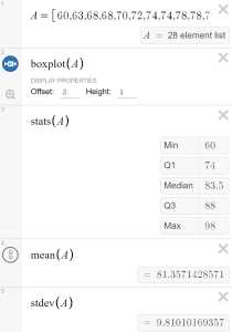
Analyzing univariate data using Desmos is now quite easy. Let your students build and explore their own data sets. Data can be either typed in as a list or imported from a spreadsheet using copy/paste. The command “Stats” provides the 5-number summary, and commands for mean and standard deviation are also available. You can play around with my dataset here.

Next, I want my students to consider transformations to the data set. In my example I have provided a list of test scores and summary statistics are provided. Let’s think about a “what if”. In the next lines I provide 2 boxplot commands, but I have intentionally ruined the command by placing an apostrophe before the command (thanks Christopher Danielson for this powerful move!). What will happen if every student is given 5 “bonus” points? What if I feel generous and add 10% to everyone’s grade?

What will happen when I remove those apostrophes? Think about the center, shape and spread of the resulting boxplots? How will these new boxplots be similar to and different from the original?

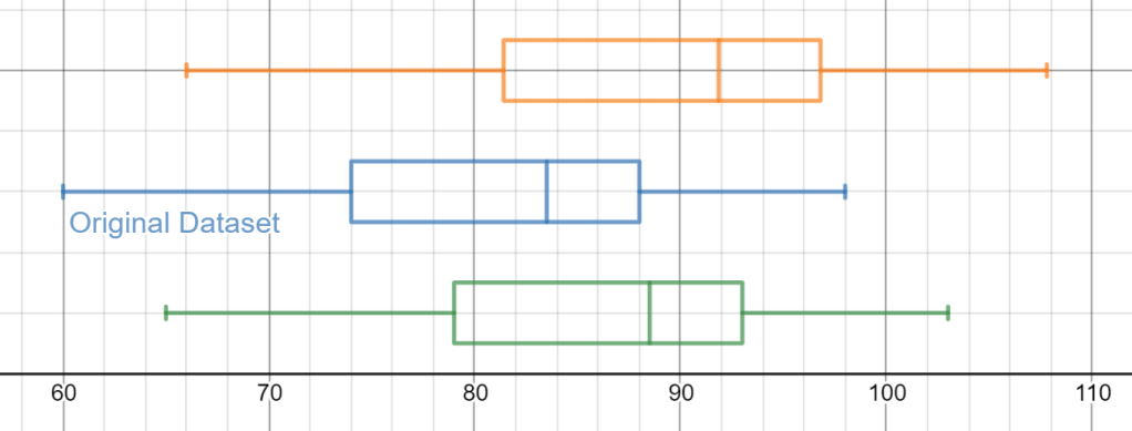
Compute new summary statistics. Which stats change…by now much…and what stays the same? Why? I’m looking forward to having students build their own linear transformation graphs, investigating and summarizing their findings! Here is a graph you can use with your classes to explore these linear transformations with sliders.

COMBINATIONS OF DISTRIBUTIONS

An important topic later in AP Stats – what happens when we combine distributions by adding or subtracting? Often I will use SAT scores as a context to introduce this topic because there are two sections (verbal and math) and a built-in need to add them – What are the total scores? On which section do students tend to do “better”…and by how much? To build a Desmos interactive here, I start with a theoretical normal distribution with mean 500 and standard deviation 100 to represent both mean and verbal score distributions. Next, taking 2 random samples of size 1000 and building commands to add and subtract them allows us to look at distributions of sums and differences and compare their center, shape and spread.

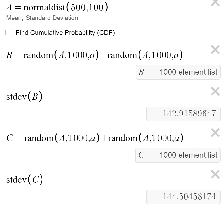
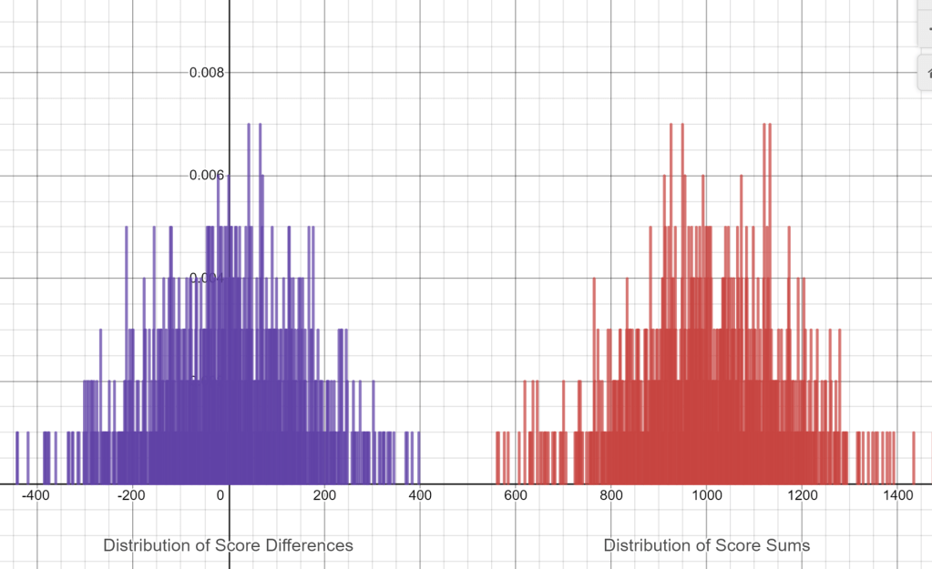
The most important take-away for students here should be that distributions of sums and differences have similar variability. This is a tricky, yet vital, idea for students as they begin to think about hypothesis tests for 2 samples. You can use my graph, or build your own. Note – in my graph the slider is used to generate repeated random samples.

Adapted from Introduction to Statistical Investigations, AP Version, by Tintle, Chance, Cobb, Rossman, Roy, Swanson and VanderStoep

Before the Thanksgiving break, I started the sampling chapter in AP Statistics.  This is a unit filled with new vocabulary and many, many class activities.  To get students thinking about random sampling, I have used the “famous” Random Rectangles activity (Google it…you’ll find it) and it’s cousin – Jelly Blubbers. These activities are effective in causing students to think about the importance of choosing a random sample from a population, and considering communication of procedures. But a new activity I first heard about at a summer session on simulation-based inference, and later explained by Ruth Carver at a recent PASTA meeting, has added some welcome wrinkles to this unit.  The unit uses the one-variable sampling applet from the Rossman-Chance applet collection, and is ideal for 1-1 classrooms, or even students working in tech teams.  Also, Beth Chance is wonderful…and you should all know that!

In my classroom notes, students first encounter the “sky”, which has been broken into 100 squares. To start, teams work to define procedures for selecting a random sample of 10 squares, using both the “hat” (non-technology) method, and a method using technology (usually a graphing calculator). Before we draw the samples however, I want students to think about the population – specifically, will a random sample do a “good job” with providing estimates? Groups were asked to discuss what they notice about the sky.  My classes immediately sensed something worth noting:

There are some squares where there are many stars (we end up calling these “dense” squares) and some where there are not so many.

Before we even drew our first sample, we are talking about the need to consider both dense and non-dense areas in our sample, and the possibility that our sample will overestimate or underestimate the population, even in random sampling.  There’s a lot of stats goodness in all of this, and the conversation felt natural and accessible to the students.

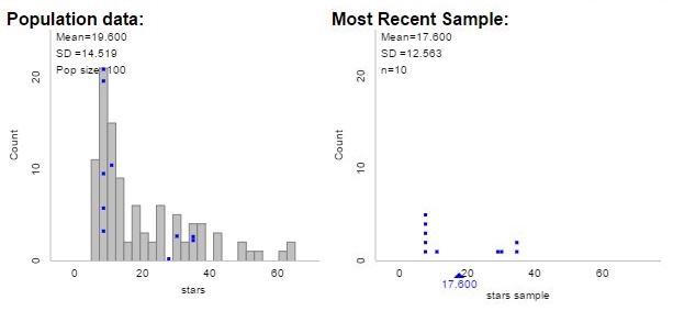
Students then used their technology-based procedure to actually draw a random sample of 10 squares, marking off the squares.  But counting the actual stars is not reasonable, given their quantity – so it’s Beth Chance to the rescue!  Make sure you click the “stars” population to get started.  Beth has provided the number of stars in each square, and information regarding density, row and column to think about later.

But before we start clicking blindly, let’s describe that population.   The class quickly agrees that we have a skewed-right distribution, and take note of the population mean – we’ll need it to discuss bias later.

Click “show sampling options” on the top of the screen and we can now simulate random samples.  First, students each drew a sample of size 10 – the bottom of the screen shows the sample, summary statistics, and a visual of the 10 squares chosen from the population.

Groups were asked to look at their sample means, share them with neighbors, and think about how close these samples generally come to hitting their target.  Find a neighbor where few “dense” area were selected , or where many “dense” squares made the cut, how much confidence do we have in using this procedure to estimate the population mean?

Eventually I unleashed the sampling power of the applet and let students draw more and more samples.  And while a formal discussion of sampling distributions is a few chapters away, we can make observations about the distributions of these sample means.

And I knew the discussion was heading in the right direction when a student observed:

Hey, the population is definitely skewed, but the means are approximately normal.  That’s odd…

Yep, it sure is…and more seeds have been planted for later sampling distribution discussions. But what about those dense and non-dense areas the students noticed earlier?  Sure, our random samples seem to provide an unbiased estimator of the population mean, but can we do better?  This is where Beth’s applet is so wonderful, and where this activity separates itself from Random Rectangles.  On the top of the applet, we can stratify our sample by density, ensuring that an appropriate ratio of dense / non-dense areas (here, 20%) is maintained in the sample.  The applet then uses color to make this distinction clear: here, green dots represent dense-area squares.

Finally, note the reduced variability in the distribution from stratified samples, as opposed to random samples. The payoff is here!

Later, we will look at samples stratified by row and/or column.  And cluster samples by row or column will also make an appearance.  There’s so much to talk about with this one activity, and I appreciate Ruth and Beth for sharing!